Intro
The fastai library
simplifies training fast and accurate neural nets using modern best
practices. See the fastai website to get started. The library is based
on research into deep learning best practices undertaken at
fast.ai, and includes “out of the box” support for
vision, text, tabular, and
collab (collaborative filtering) models.
Tabular
Tabular data can be downloaded from Kaggle. It is a basic binary classification case which contains both categorical and coninuous columns. Below one can see the structure of the dataset.
library(magrittr)
library(fastai)
df = data.table::fread('datasets_236694_503227_HR_comma_sep.csv')
str(df)
> str(df)
Classes ‘data.table’ and 'data.frame': 14999 obs. of 10 variables:
$ satisfaction_level : num 0.38 0.8 0.11 0.72 0.37 0.41 0.1 0.92 0.89 0.42 ...
$ last_evaluation : num 0.53 0.86 0.88 0.87 0.52 0.5 0.77 0.85 1 0.53 ...
$ number_project : int 2 5 7 5 2 2 6 5 5 2 ...
$ average_montly_hours : int 157 262 272 223 159 153 247 259 224 142 ...
$ time_spend_company : int 3 6 4 5 3 3 4 5 5 3 ...
$ Work_accident : int 0 0 0 0 0 0 0 0 0 0 ...
$ left : int 1 1 1 1 1 1 1 1 1 1 ...
$ promotion_last_5years: int 0 0 0 0 0 0 0 0 0 0 ...
$ sales : chr "sales" "sales" "sales" "sales" ...
$ salary : chr "low" "medium" "medium" "low" ...
- attr(*, ".internal.selfref")=<externalptr> Output column is left which is integer. Output has to be
converted to character/factor.
df[['left']] = as.factor(df[['left']])Later, we need to divide column names into 2 groups:
- Categorical columns
- Continuous columns
dep_var = 'left'
cat_names = c('sales', 'salary')
cont_names = c("satisfaction_level", "last_evaluation", "number_project",
               "average_montly_hours", "time_spend_company",
               "Work_accident", "promotion_last_5years")
Alternatively, it is easier to differentiate 2 types of columns
(integer/numeric vs. character/factor) with
dplyr::select_if(is.character).
Next step is to split data into 2 parts. However, we need to randomly
select indices not rows because the latter will be done by
tabular_learner.
The dataset can contain missing/large values. Therefore,
fill missing and normalize functions from
fastai can quickly handle these situations.
procs = list(FillMissing(),Categorify(),Normalize())In addition, filling missing values can be done in different ways:
- filling value by default is 0
- or it can be set to median
Dataloaders
Define data loaders and specify batch_size,
cat_names, cont_names and etc:
dls = TabularDataTable(df, procs, cat_names, cont_names,
                       y_names = dep_var, splits = list(tr_idx, ts_idx) ) %>%
  dataloaders(bs = 50)
A deep learning model which contains embedding layers for categorical columns and linear for continuous ones. At the same time, define metrics:
model = dls %>% tabular_learner(layers=c(200,100,100,200),
                                config = tabular_config(embed_p = 0.3, use_bn = FALSE),
                                metrics = list(accuracy, RocAucBinary(),
                                             Precision(), Recall(),
                                             F1Score()))
> model
TabularModel(
(embeds): ModuleList(
(0): Embedding(11, 6)
(1): Embedding(4, 3)
)
(emb_drop): Dropout(p=0.3, inplace=False)
(bn_cont): BatchNorm1d(7, eps=1e-05, momentum=0.1, affine=True, track_running_stats=True)
(layers): Sequential(
(0): LinBnDrop(
(0): Linear(in_features=16, out_features=200, bias=True)
(1): ReLU(inplace=True)
)
(1): LinBnDrop(
(0): Linear(in_features=200, out_features=100, bias=True)
(1): ReLU(inplace=True)
)
(2): LinBnDrop(
(0): Linear(in_features=100, out_features=100, bias=True)
(1): ReLU(inplace=True)
)
(3): LinBnDrop(
(0): Linear(in_features=100, out_features=200, bias=True)
(1): ReLU(inplace=True)
)
(4): LinBnDrop(
(0): Linear(in_features=200, out_features=2, bias=True)
)
)
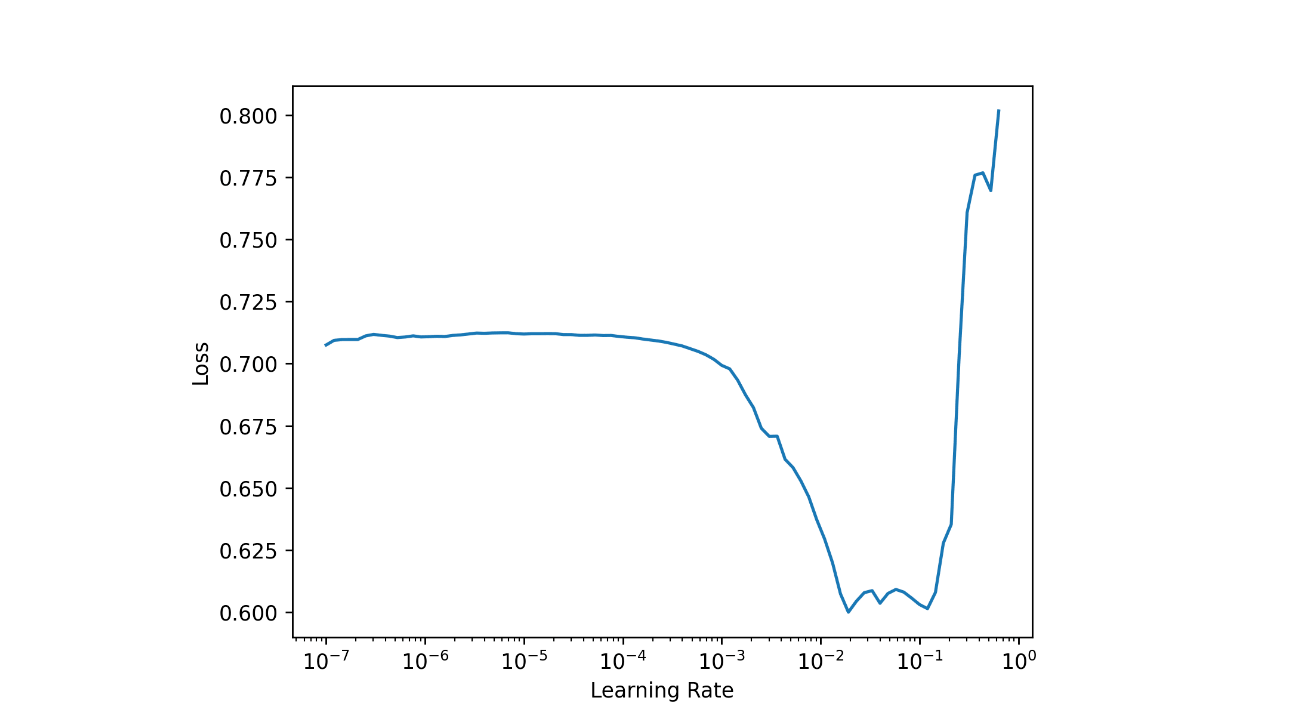
)Before fitting model find optimal learning rate:
lrs = model %>% lr_find()
# SuggestedLRs(lr_min=0.002754228748381138, lr_steep=1.5848931980144698e-06)

model %>% plot_lr_find()
Fit
And finally, fit the model:
epoch     train_loss  valid_loss  accuracy  roc_auc_score  precision_score  recall_score
0         0.173383    0.189803    0.950333  0.969118       0.900000         0.893793
1         0.151623    0.132094    0.960000  0.980776       0.924264         0.908966
2         0.154831    0.118114    0.963333  0.984218       0.939914         0.906207
3         0.149708    0.127625    0.958667  0.982307       0.916782         0.911724
4         0.132304    0.103252    0.967667  0.986488       0.964497         0.899310
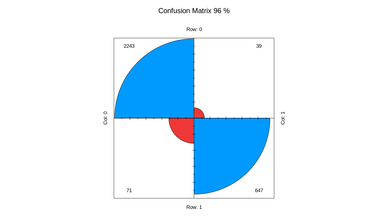
Plot confusion matrix:
model %>% get_confusion_matrix() %>%
  fourfoldplot(conf.level = 0, color = c("#ed3b3b", "#0099ff"),
             margin = 1,main = paste("Confusion Matrix",
                                     round(sum(diag(.))/sum(.)*100,0),"%",sep = ' '))
Conclusion
Let’s make predictions:
        0           1         class
1  0.004488660 0.99551141       1
2  0.819206953 0.18079305       0
3  0.051526461 0.94847351       1
4  0.003814965 0.99618500       1
5  0.007526034 0.99247390       1
6  0.093833014 0.90616697       1
7  0.910625637 0.08937429       0
8  0.005479155 0.99452078       1
9  0.025799874 0.97420007       1
10 0.103506751 0.89649332       1
11 0.068529680 0.93147027       1