Head pose • fastai

Intro

The fastai library simplifies training fast and accurate neural nets using modern best practices. See the fastai website to get started. The library is based on research into deep learning best practices undertaken at fast.ai, and includes “out of the box” support for vision, text, tabular, and collab (collaborative filtering) models.

Task

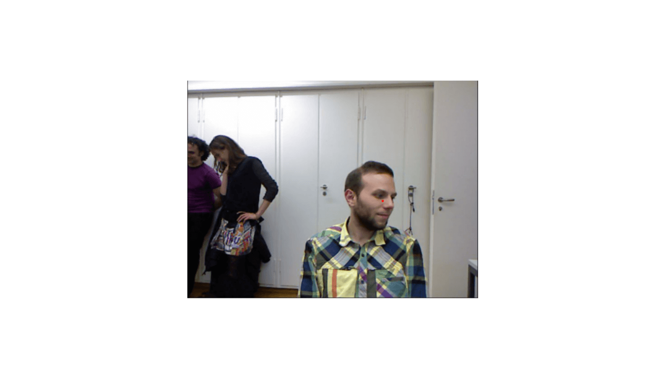
Our task is to find the center of the head in each image.

To achieve the goal, we need to do the following:

upload images with DataBlock
add red points to the images

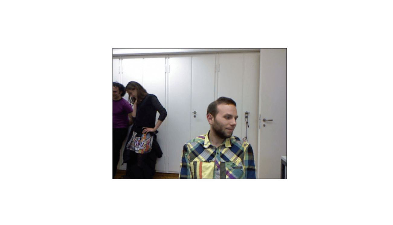
Upload an example:

library(fastai)
library(magrittr)

path = 'biwi_head_pose'
fname = '09/frame_00667_rgb.jpg'

img = Image_create(paste(path,fname,sep = '/'))
img %>% show() %>% plot()
cal = readr::read_lines(paste(path,'01/rgb.cal',sep = '/'), n_max = 3) %>% trimws() %>%
  strsplit('\\s') %>% do.call(rbind,.) %>% apply(.,2,as.numeric)

To add the points, we need to write simple functions:

img2txt_name <- function(f) {
  paste(
    substr(f, 1, nchar(f)-7), 'pose.txt',
    sep = ''

  )
}

convert_biwi <- function(coords) {
  c1 = coords[1] * cal[1,][1]/coords[3] + cal[1,][3]
  c2 = coords[2] * cal[2,][2]/coords[3] + cal[2,][3]
  return(tensor(c1,c2))
}

get_ctr <- function(f) {
  # trick to make dataloaders work
  f = as.character(f)
  ctr = readr::read_lines(img2txt_name(f), skip = 4, n_max = 1) %>% trimws() %>%
    strsplit('\\s') %>% unlist() %>% as.numeric()
  convert_biwi(ctr)
}

get_ip <- function(img, pts) {
  TensorPoint_create(pts, img_size = img$size)
}

ctr = readr::read_lines(img2txt_name(paste(path,fname,sep = '/')),
                        skip = 4, n_max = 1) %>% trimws() %>%
      strsplit('\\s') %>% unlist() %>% as.numeric()

Now, it is easier to add red points:

ctr = get_ctr(paste(path,fname,sep = '/'))
ax = img %>% show(figsize = c(6, 6))
img %>% get_ip(ctr) %>% show(ctx = ax) %>% plot()

Preparation

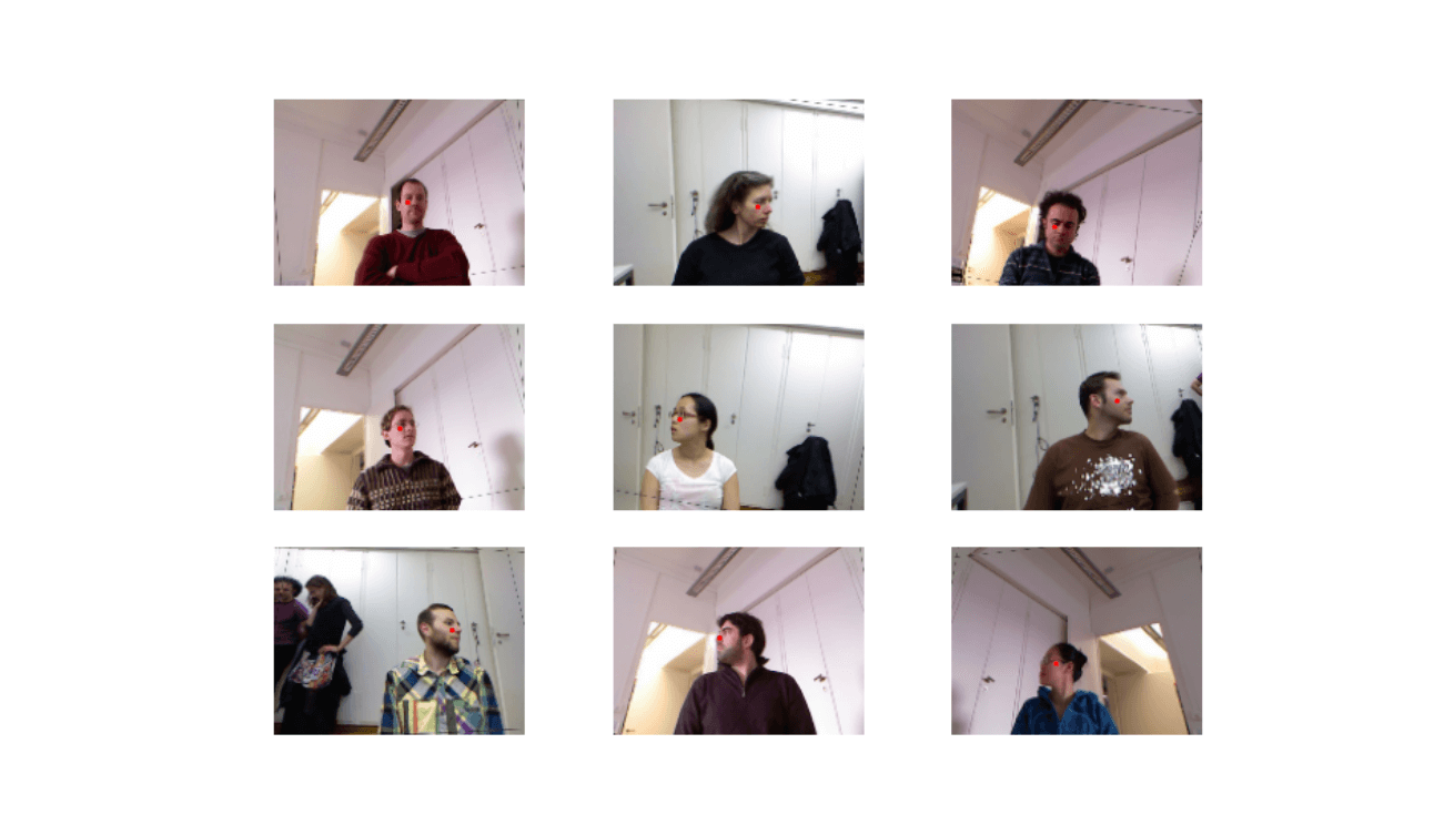
Prepare data laoder object and see batch:

dblock = DataBlock(blocks = list(ImageBlock(), PointBlock()),
                   get_items = get_image_files(),
                   splitter = FuncSplitter(function(x) x$parent$name == '13'),
                   get_y = get_ctr,
                   batch_tfms = list(aug_transforms(size = c(120,160)),
                                     Normalize_from_stats(imagenet_stats()
                                                          )
                                     )
                   )

dls = dblock %>% dataloaders(path, path = path, bs = 64)

dls %>% show_batch(max_n = 9, figsize = c(9,6))

Fit

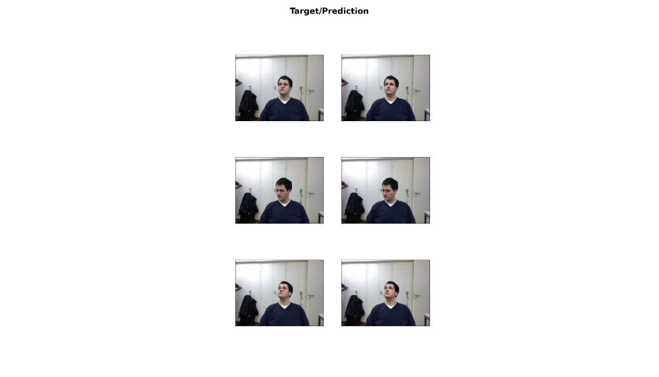
Run for 5 epochs and see results:

learn = cnn_learner(dls, resnet34())

learn %>% lr_find()

learn %>% plot_lr_find()

lr = 2e-2

learn %>% fit_one_cycle(5, slice(lr))

learn %>% show_results(dpi = 200)

epoch     train_loss  valid_loss  time    
0         1.818259    0.861968    00:35     
1         0.222080    0.056300    00:34     
2         0.028511    0.012499    00:33     
3         0.017333    0.003378    00:33     
4         0.015135    0.004777    00:33